The NAS benchmark MG implements a V-cycle multigrid algorithm to approximate a solution u of the discrete Poisson equation $\nabla^2 u = v$ on a 3-dimensional grid with periodic boundary conditions. Rather than iteratively applying relaxation steps to a grid of fixed size as in the PDE1 benchmark, they are consecutively applied to grids of varying granularity, i.e., they are embedded within operations to coarsen and refine grids. The rationale for this approach is to accelerate the propagation of low-frequent defects across the original grid and, hence, to improve the convergence behaviour.

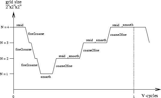
The Mgrid benchmark iteratively applies a V-cycle multigrid relaxation algorithm to a 3-dimensional grid. A single V-cycle consists of a recursive nesting of relaxation steps and smoothing steps on grids of varying granularity as well as of mappings between these grids. The figure and the SAC-code below illustrate a single V-cycle for a grid of $64^3$ elements. The order in which the different transformations are applied is depicted along the horizontal axis, whereas the grid size involved in each step is indicated along the vertical axis.

Illustration of multigrid V-cyle

Following a top-down approach, this sequence of operations can easily be implemented by means of the two functions MGrid and VCycle shown in the SAC-code below. MGrid creates the initial solution grid u before it alternatingly computes the current residual and the correction of the current solution by means of a single V-cycle. The recursive function VCycle realizes exactly the sequence of basic operations, as is illustrated in the figure above. Both implementations almost literally coincide with their mathematical specifications.

double[+] MGrid( double[+] v, int iter)
{
  u = genarray( shape(v), 0d);
 
  for( i=0; i<iter; i+=1)
  {
    r = v - Resid( u);
    u = u + VCycle( r);
  }
 
  return( u);
}
 
double[+] VCycle( double[+] r)
{
  if (Coarsest( r))
  {
    z = Smooth( r);
  }
  else
  {
    rn = Fine2Coarse( r);
    zn = VCycle( rn);
    z  = Coarse2Fine( zn);
    r  = r - Resid( z);
    z  = z + Smooth( r);
  }
 
  return( z);
}

Whereas arithmetic array operations used in the definitions of MGrid and VCycle are just imported from the SAC array library, additional implementations are required for relaxation and smoothing operations as well as for the mappings between grids of different size. A closer look at their specifications reveals that they uniformly contain single relaxation steps, which only vary with respect to weights associated with adjacent elements.

Introducing artificial boundary elements

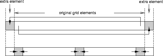
Implementing relaxation steps in SAC has already been addressed in PDE 1 Implementation. But whereas the PDE1 benchmark is characterized by fixed boundary conditions, NAS-MG uses periodic ones, i.e., the grid represents a torus rather than a cube. A solution which still allows for reuse of existing code is to artificially extend the original grid by additional boundary elements. More precisely, each original boundary element is replicated on the opposite side of the grid, as illustrated in the figure above. They allow to implement relaxation with periodic boundary conditions by two consecutive steps.

1. Artificial boundary elements are initialized according to their location.
2. An ordinary relaxation step is applied to the extended grid.

double[+] Resid( double[+] u)
{
  u = SetupPeriodicBorder( u);
  u = RelaxKernel( u, A);
 
  return( u);
}
 
double[+] Smooth( double[+] r)
{
  r = SetupPeriodicBorder( r);
  r = RelaxKernel( r, S);
 
  return( r);
}

Based on the existing relaxation kernel as developed for the PDE1 benchmark, the four V-cycle operations can be implemented more or less straightforwardly. As shown in the code, implementations of Resid and Smooth boil down to setting up the periodic boundary elements followed by a single relaxation step. In fact, they only differ with respect to the weights associated with adjacent elements during the relaxation step. However, A and S are constant arrays defined by the benchmark specification.

double[+] Fine2Coarse( double[+] r)
{
  rs = SetupPeriodicBorder( r);
  rr = RelaxKernel( r, P);
  rc = condense( 2, rr);
  rn = embed( shape(rc)+1, 0*shape(rc), rc);
 
  return( rn);
}
 
double[+] Coarse2Fine( double[+] rn)
{
  rp = SetupPeriodicBorder( rn);
  rs = scatter(2, rp);
  rt = take( shape(rs)-2, rs);
  r  = RelaxKernel( rt, Q);
 
  return( r);
}

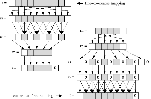
Implementations of the remaining V-cycle functions Fine2Coarse and Coarse2Fine are shown above. Besides applying additional relaxation steps similar to Resid and Smooth, but with yet different weights P and Q, they map fine grids to coarse grids and vice versa, as illustrated in the next figure. Both mapping steps can be realized by combinations of predefined array operations from the SAC library, whose implementations are shown in the code below.

Illustration of mapping steps

The fine-to-coarse mapping is basically implemented by means of the function condense (str, a), which creates an array whose extent in each dimension is by a factor of str less than that of the given array a. Its elements are taken from applying a stride of str. However, due to the additional boundary elements, condense does not exactly match the fine-to-coarse mapping requirements, as the result array lacks one such element . Therefore, the intermediate array rc must subsequently be embedded into an array of correct size. This is specified by means of the library function embed( shp, pos, a), which creates a new array of shape shp, whose elements starting at index position pos are copied from the argument array a. Actually, the function embed is complementary to the function tile used for the specification of the relaxation kernel in PDE 1 Implementation.

The coarse-to-fine mapping is implemented by means of the library function scatter(str, a), which is complementary to condense. As illustrated , it creates an array which in each dimension is by a factor of str larger than the given array a. All elements of a are copied into every other location of the result array applying the given stride str; remaining elements are initialized by 0. However, due to the additional boundary elements, the resulting array is by two elements too large in each dimension; a subsequent application of the library function take removes them.

double[+] condense( int str, double[+] a)
{
  ac = with (. <= iv <= .)
       genarray( shape(a) / str, a[str*iv]);
 
  return( ac);
}
 
double[+] scatter( int str, double[+] a)
{
  as = with (. <= iv <= . step str)
       genarray( str * shape(a), a[iv/str]);
 
  return( as);
}
 
double[+] embed( int[.] shp, int[.] pos, double[+] a)
{
  ae = with (pos <= iv < shape(a)+pos)
       genarray( shp, a[iv-pos]);
 
  return( ae);
}
 
double[+] take( int[.] shp, double[+] a)
{
  at = with (. <= iv <= .)
       genarray( shp, a[iv]);
 
  return( at);
}